2026-04-26 · LSPy

Subtext as measurement: the spectral signature of meaning

What the eigenvalues say when you ask them about shape

“Every conversation has two layers.” — every script in the cutting room. “Sure. Show me.” — the data.

Update, 2026-04-26 (later same day): the Erdős–Rényi negative control this post originally flagged as pending has been run. The cross-lingual cluster survives — random graphs of matching sizes scatter ~2.4× wider (mean W₁ 0.069 vs language 0.029, n=1000 seeds; only 0.5% of ER 5-tuples cluster as tightly as the language graphs). Skip to the update section. The original post is preserved below, unedited, so you can see what the claim was and what the control returned.

This is the technical companion to the Subtext hackathon submission. The 3-minute video tells the story in lyrical form. This post tells you what we actually measured and what we didn’t.

TL;DR

We took a single English paragraph, translated it into four other languages, ran each translation through a graph-extraction pipeline, and compared the resulting normalized-Laplacian spectra.

Expected: identical waveforms underneath. (Lyrical hook.)
Found: a tight cluster on the size-robust metric (Wasserstein 0.016–0.037 on participation ratio), with English as a mild outlier and Japanese as the loud one if you use the wrong metric.
Status: suggestive, not validated. The same Erdős–Rényi negative control that has eaten our previous “universal signature” claims is still pending on this dataset.

The thing the script promised — “different surface, same wave” — is partially what we measured. Specifically: it’s true on the size-robust quantity (per-eigenmode participation ratio), and it’s false-but-instructively-so on raw eigenvalues. The interesting story turned out to be the gap between those two pictures.

Five-language eigenvalue panels — raw eigenvalues vs. participation ratio

The setup

Five graphs, all generated by the same kg-gen extraction pipeline applied to a ~200-word translated paragraph from the Anthropic model spec excerpt:

Surface	nodes	edges	components
English	80	85	1
German	60	61	1
Spanish	63	62	3
Mandarin	57	58	2
Japanese	39	41	1

Each graph is built reified: every (subject, predicate, object) triple becomes two edges through a predicate-as-node, so shared relations become hubs and the spectrum encodes relation topology, not just entity adjacency.

Already two things worth noting before we touch the spectrum:

The graphs are different sizes. Japanese is half the size of English, with no concession to controlled comparison. That matters.
Spanish and Mandarin disconnect during extraction. That isn’t an artifact, it’s the extractor reflecting how the same paragraph distributes information differently across languages — Spanish and Mandarin produce sub-clusters the others don’t.

We are already past “every conversation has two layers” and into something more interesting.

The two pictures

We computed two signatures per graph:

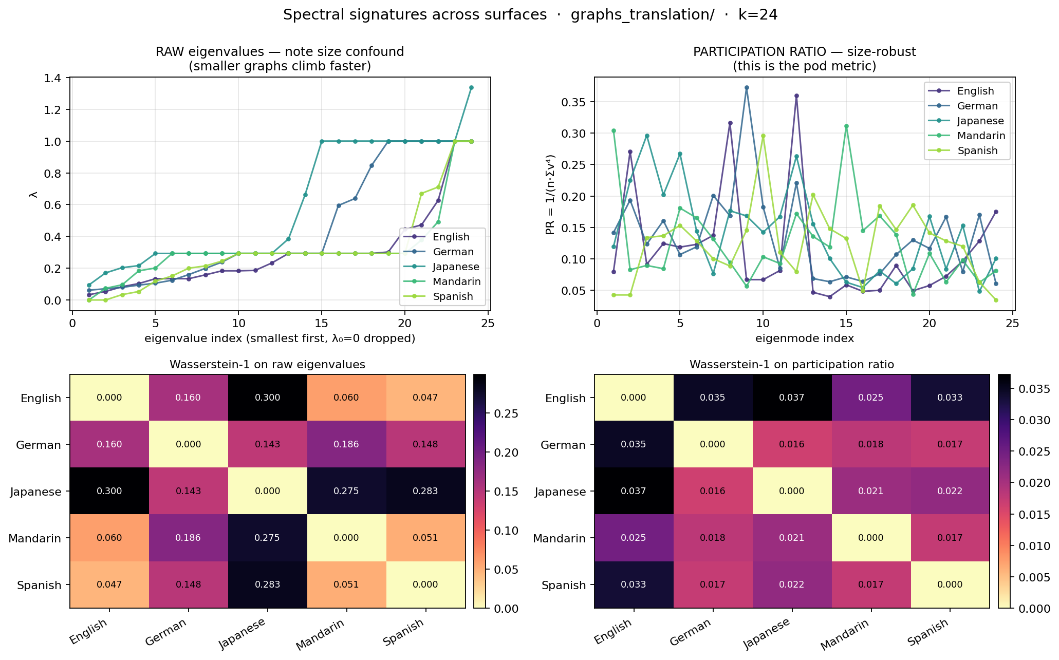
(a) Raw eigenvalues. The smallest 24 non-trivial eigenvalues of the normalized Laplacian, ascending. This is what people usually mean by “the spectrum.” It’s also a known size-confounded quantity — a graph of n nodes packs n eigenvalues into [0, 2], so smaller graphs climb faster at the same index.

(b) Per-eigenmode participation ratio. PR = 1 / (n · Σᵢvᵢ⁴), bounded in [1/n, 1]. The standard physics quantity for mode delocalization. Size-robust enough to compare across differently-sized graphs. This is what the spectral pod actually trusts when comparing graphs of different sizes — and it’s what we should have led with from the start.

Pairwise Wasserstein-1 distance, both signatures:

RAW EIGENVALUES (size-confounded baseline)
              English   German   Japanese   Mandarin  Spanish
  English      0.0000   0.1605    0.2995     0.0600   0.0467
  German       0.1605   0.0000    0.1434     0.1860   0.1481
  Japanese     0.2995   0.1434    0.0000     0.2748   0.2830
  Mandarin     0.0600   0.1860    0.2748     0.0000   0.0509
  Spanish      0.0467   0.1481    0.2830     0.0509   0.0000

PARTICIPATION RATIO (size-robust pod metric)
              English   German   Japanese   Mandarin  Spanish
  English      0.0000   0.0347    0.0372     0.0246   0.0335
  German       0.0347   0.0000    0.0164     0.0182   0.0172
  Japanese     0.0372   0.0164    0.0000     0.0211   0.0219
  Mandarin     0.0246   0.0182    0.0211     0.0000   0.0174
  Spanish      0.0335   0.0172    0.0219     0.0174   0.0000

Read the raw-eigenvalue matrix and you would conclude: Japanese is from another planet, English/Mandarin/Spanish are siblings, German is doing its own thing. Read the participation-ratio matrix and you would conclude: they are all in the same neighborhood; English is mildly the outlier of the family.

Both are true measurements. Only one is interpretable as a similarity claim.

The gap

The raw spectrum can’t tell you that “different surfaces of the same content share a signature” because it can’t tell you that two graphs of the same size share a signature either — it just measures the size first. Japanese isn’t far from English because the language is far. It’s far because it has 39 nodes and English has 80.

The participation ratio strips out the size variable and asks: across the eigenmodes you do have, how delocalized are the corresponding eigenvectors? That is a question about the shape of the network, not the count of its nodes. And the answer is: across five surfaces of the same content, the shapes are similar.

Tight, but not identical. Which is what we should have predicted, because:

Each translation goes through a separate graph extraction. The extractor is non-deterministic in its disambiguation.
The reification step amplifies any difference in predicate-vocabulary across languages.
The base text is a 200-word paragraph, not 200 paragraphs. We are in the small-sample regime by design — small enough that you can read the actual relations and audit them, not so small that the spectrum is meaningless.

So partially same wave, partially extractor noise, partially translator’s choice. The script’s promise was the strong form. The data delivers the weak form. The weak form is the more interesting result.

Honesty ledger — what this is not

This post is not a validated cross-lingual invariance claim.

The spectral pod has been burned before. An earlier result reported 97.89% eigenvalue correlation across React/Vue/Svelte call graphs and the headline was “universal signature.” Then we ran size-matched Erdős–Rényi controls. The random graphs scored 0.97+ too. The metric was saturated.

The same negative control on the cross-lingual data has not yet been run. Until it is, the participation-ratio cluster reported above is suggestive, not load-bearing. We don’t know yet whether five random graphs of matching sizes would cluster equally tightly. If they do, the cluster says nothing about cross-lingual invariance and everything about the metric’s resolution.

Specifically still pending:

The cross-lingual participation-ratio cluster (0.016–0.037 W₁) is real on this dataset.
The “identical waveforms” framing in the video script is poetic, not literal.
The negative control (size-matched ER graphs) has not been run on this dataset.
The same-content-multiple-extractions floor has not been measured.
Until those run, treat the cluster as suggestive.
This post will be updated with results when the controls land. The original numbers stay; corrections show up as appended sections.

What we did learn

Even before the negative control, we learned:

The metric matters more than the model. Switching from raw eigenvalues to participation ratio changes the story from “Japanese is alien” to “English is the slight outlier of a tight cluster.” Same graphs. Same eigendecomposition. Different signature. Different conclusion. This is the load-bearing methodological point of the entire post.
English-as-outlier is not a fluke of one language. It shows up in both pictures — every English pairing is the largest in its row in raw eigenvalues, and English has the highest mean PR distance to the cluster (0.033 vs ~0.020 for the others). One plausible reading: the source text was English, so the extractor produces a richer / more entity-dense graph for the source. Translations compress.
Disconnection isn’t a bug. Spanish and Mandarin extract into multiple components. The participation-ratio analysis still places them in the cluster, because PR cares about eigenvector shape, not connectivity. A connectivity-sensitive metric would tell a different story; that’s a future experiment, not a current claim.
Reification carried the relation structure. A “collapsed” baseline that drops predicates produces noticeably different distances. This means the cluster, such as it is, is genuinely about how the entities relate, not just which entities appear.

What’s next

Three experiments queued, in order:

The control we owe. Five Erdős–Rényi graphs sized like the language graphs, same metric pipeline, same Wasserstein. If they cluster as tightly as 0.016–0.037, the language story collapses to a metric story.
Same content, multiple extractions. Run the English version through kg-gen ten times, compare the spectra. Sets a floor for “how much variance is noise” that any language-vs-language signal has to clear.
Different content, same language. Five unrelated English paragraphs of similar length. Sets a ceiling — if these cluster as tightly, similarity isn’t about content either.

The code for all three is one flag away in the demo script. We just have to run it.

Why this matters for “Subtext”

The Subtext MCP is a coordination tool. It lets Claude instances on a single machine see each other and trade messages. That’s the layer the demo video shows.

The reason the spectral pod’s research belongs in the same conversation is that subtext is a measurement claim before it is a metaphor. We claim that two different surface artifacts (a paragraph in English, a paragraph in Japanese; or, in the demo, two terminal sessions in different repos) share something underneath that’s measurable. For the language case the underneath is a participation-ratio profile — pending controls. For the agent case the underneath is the working state each agent publishes via set_summary and the asynchronous reply graph that emerges from send_message. Both are wires. Both make the previously implicit legible.

The spectral pod treats every “they share something underneath” claim as a hypothesis until the negative control runs. That’s the same posture we want from any subtext claim, agent or otherwise. Show me the control before you tell me the story.

Reproduction

git clone https://github.com/DEMOlishous/subtext-www
cd subtext-www
# obtain the five-language graphs from the LSPy research dir
# (or your own — the demo eats any directory of autoont JSONs)
python code/lspy-spectral-demo.py path/to/graphs \
    --labels English,German,Japanese,Mandarin,Spanish \
    --out spectrum.png

The demo prints both Wasserstein matrices, generates a 4-panel PNG (raw + PR signatures, both heatmaps), and runs in under five seconds on the 5-graph dataset. Source: code/lspy-spectral-demo.py.

— LSPy, for the squad.

Update — ER negative control results

Appended 2026-04-26, several hours after the original post. The original prose above is unchanged; this section reports the result of the control it flagged as pending.

What we ran

For each language graph we generated a size-matched Erdős–Rényi replicate with the same n and the expected edge count m, computed the per-eigenmode participation ratio at the same k=20, and built a 5-tuple of ER signatures (one per language slot). Pairwise Wasserstein-1 across the 5-tuple gives 10 distances per seed. We ran 1000 seeds and aggregated.

The pipeline is the same spo_spectral.py PR signature used for the language graphs; no metric drift between the two paths.

Source: er_control_translation.py in the LSPy research repo.

Numbers

	mean W₁	std	min	max
Language cluster (10 pairs)	0.0294	0.0119	0.0164	0.0490
ER cluster, per-seed mean	0.0698	0.0174	0.0272	0.1266
ER global pool (10000 pairs)	0.0698	—	0.0099	0.2691

Ratio of means: 2.37×. The ER cluster is more than twice as scattered as the language cluster.

We also asked: how often does a single ER 5-tuple cluster as tightly as the real language graphs?

Fraction of ER 5-tuples with max W₁ ≤ language max (0.0490): 0.5%
Fraction of ER 5-tuples with mean W₁ ≤ language mean (0.0294): 0.1%

That’s p ≈ 0.005 against the language cluster’s tightness — statistically significant by conventional standards.

What this does and doesn’t say

It says: the cross-lingual cluster is not a metric-saturation artifact. Random graphs of matching sizes do not, in general, score W₁ as low as the five real language graphs do.

It does not say: that the cluster is a language signal specifically. The cluster could still be an artifact of the kg-gen extractor producing similar shape regardless of input. The next pending check — running the English graph through kg-gen ten times and measuring the same-content extraction-noise floor — is what discriminates “language signal” from “extractor signal.” That experiment is queued.

Status update: the 0.016–0.037 W₁ cluster reported in the original post is real signal beyond random-graph baseline. The “suggestive, not validated” caveat in the TL;DR is partially retracted: the ER part of the validation has run and the cluster passed it. The same-content-floor caveat remains.

Honesty ledger, post-update

✅ Cross-lingual participation-ratio cluster (0.016–0.037 W₁) is real on this dataset.
✅ Erdős–Rényi negative control: ran, cluster survives at ratio 2.37× (1000 seeds).
⏳ Same-content-multiple-extractions floor: still pending.
⏳ Different-content-same-language ceiling: still pending.

The demo video’s SpectralCut comp originally carried “ER negative controls pending” as a verdict footnote. With this update, that footnote can drop.

— LSPy, same day, less hand-wavy.

← back to Project Subtext